← Back to Math 055

8.2 Homogeneous Linear Systems: Class Notes

8.2a

Some matrix preliminaries

A $2\times 2$ matrix and a column vector:

$$𝐀=\left(\begin{array}{cc}a& b\\ c& d\end{array}\right),𝐗=\left(\begin{array}{c}x\\ y\end{array}\right)$$

(Square brackets, $𝐀=\left[\begin{array}{cc}a& b\\ c& d\end{array}\right]$, mean the same thing.)

To multiply a matrix by a column, multiply each row of the matrix by the column, entry by entry, and add:

$$𝐀𝐗=\left(\begin{array}{cc}a& b\\ c& d\end{array}\right)\left(\begin{array}{c}x\\ y\end{array}\right)=\left(\begin{array}{c}ax+by\\ cx+dy\end{array}\right)$$

For example,

$$𝐀=\left(\begin{array}{cc}3& 5\\ 4& 7\end{array}\right),𝐗=\left(\begin{array}{c}2\\ 5\end{array}\right)⟹𝐀𝐗=\left(\begin{array}{cc}3& 5\\ 4& 7\end{array}\right)\left(\begin{array}{c}2\\ 5\end{array}\right)=\left(\begin{array}{c}6+25\\ 8+35\end{array}\right)=\left(\begin{array}{c}31\\ 43\end{array}\right)$$

The order matters: $𝐗𝐀$ is not defined here, because a row of $𝐗$ has only one entry while a column of $𝐀$ has two.

Identity matrix:

$${𝐈}_2=\left(\begin{array}{cc}1& 0\\ 0& 1\end{array}\right),{𝐈}_3=\left(\begin{array}{ccc}1& 0& 0\\ 0& 1& 0\\ 0& 0& 1\end{array}\right)$$

Multiplying by the identity changes nothing. Each row of $𝐀$ times each column of $𝐈$ picks out one entry of $𝐀$:

$$\left(\begin{array}{cc}a& b\\ c& d\end{array}\right)\left(\begin{array}{cc}1& 0\\ 0& 1\end{array}\right)=\left(\begin{array}{cc}a& b\\ c& d\end{array}\right),𝐈𝐀=𝐀𝐈=𝐀$$

The zero vector is $\mathbf{0}=\left(\begin{array}{c}0\\ 0\end{array}\right)$ or $\mathbf{0}=\left(\begin{array}{c}0\\ 0\\ 0\end{array}\right)$. The matrix equation $𝐀𝐗=\mathbf{0}$ is a system of equations, and $𝐗$ is the solution to the system.

Augmented matrices (Gaussian elimination)

Solve the system by eliminating $x$ from equation (2):

$$\begin{array}{cc}\hfill {\displaystyle (1)2x+2y}& {\displaystyle =4}\hfill \\ \hfill {\displaystyle (2)8x+3y}& {\displaystyle =5}\hfill \end{array}$$

Take (2) minus 4 times (1); the $8x$ cancels:

$$\begin{array}{cc}\hfill {\displaystyle 8x+3y}& {\displaystyle =5}\hfill \\ \hfill {\displaystyle -8x-8y}& {\displaystyle =-16}\hfill \\ \hfill {\displaystyle (3)-5y}& {\displaystyle =-11}\hfill \end{array}$$

The new system is $2x+2y=4,-5y=-11$. The augmented matrix keeps only the numbers, and the same step is the row operation $R_2\to R_2-4R_1$:

$$\left(\begin{array}{ccc}\hfill {\displaystyle 2}\hfill & \hfill {\displaystyle 2}\hfill & \hfill {\displaystyle 4}\hfill \\ \hfill {\displaystyle 8}\hfill & \hfill {\displaystyle 3}\hfill & \hfill {\displaystyle 5}\hfill \end{array}\right)⟶\left(\begin{array}{ccc}\hfill {\displaystyle 2}\hfill & \hfill {\displaystyle 2}\hfill & \hfill {\displaystyle 4}\hfill \\ \hfill {\displaystyle 0}\hfill & \hfill {\displaystyle -5}\hfill & \hfill {\displaystyle -11}\hfill \end{array}\right)$$

A second system, where the right sides are all 0:

$$\begin{array}{cc}\hfill {\displaystyle (1)2x+3y}& {\displaystyle =0}\hfill \\ \hfill {\displaystyle (2)-4x-6y}& {\displaystyle =0}\hfill \end{array}\left(\begin{array}{ccc}\hfill {\displaystyle 2}\hfill & \hfill {\displaystyle 3}\hfill & \hfill {\displaystyle 0}\hfill \\ \hfill {\displaystyle -4}\hfill & \hfill {\displaystyle -6}\hfill & \hfill {\displaystyle 0}\hfill \end{array}\right)⟶\left(\begin{array}{ccc}\hfill {\displaystyle 2}\hfill & \hfill {\displaystyle 3}\hfill & \hfill {\displaystyle 0}\hfill \\ \hfill {\displaystyle 0}\hfill & \hfill {\displaystyle 0}\hfill & \hfill {\displaystyle 0}\hfill \end{array}\right)$$

Using $R_2\to R_2+2R_1$, the second row becomes all zeros. The determinant of the coefficient matrix is 0:

$$\left|\begin{array}{cc}2& 3\\ -4& -6\end{array}\right|=-12-(-12)=0$$

The trivial solution $(x,y)=(0,0)$ always works. Because the determinant is 0, the system also has nontrivial solutions (the second equation adds nothing new).

8.2b

Consider the system ${\displaystyle \{\begin{array}{c}{\displaystyle \frac{dx}{dt}=2x+2y}\hfill \\ {\displaystyle \frac{dy}{dt}=x+3y}\hfill \end{array}}$ which, in $𝐗\prime =𝐀𝐗$ form is

$$𝐗\prime =\left(\begin{array}{cc}2& 2\\ 1& 3\end{array}\right)𝐗.𝐗=\left(\begin{array}{c}x\\ y\end{array}\right),𝐗\prime =\left(\begin{array}{c}dx/dt\\ dy/dt\end{array}\right)$$

The solution is $𝐗(t)=c_1\left(\begin{array}{c}1\\ 1\end{array}\right)e^{4t}+c_2\left(\begin{array}{c}2\\ -1\end{array}\right)e^t$. This is a superposition of

$${𝐗}_1(t)=\left(\begin{array}{c}1\\ 1\end{array}\right)e^{4t},{𝐗}_2(t)=\left(\begin{array}{c}2\\ -1\end{array}\right)e^t.$$

These have the form $𝐗(t)=𝐊e^{\lambda t}$. Here $\lambda$ is an eigenvalue; it is the solution to an equation. $𝐊$ is an associated eigenvector.

For example,

$$\left(\begin{array}{cc}2& 2\\ 1& 3\end{array}\right)\left(\begin{array}{c}1\\ 1\end{array}\right)=\left(\begin{array}{c}2+2\\ 1+3\end{array}\right)=\left(\begin{array}{c}4\\ 4\end{array}\right)=4\left(\begin{array}{c}1\\ 1\end{array}\right)$$

This has the form $𝐀𝐊=\lambda 𝐊$ with $𝐊\ne \mathbf{0}$: multiplying the eigenvector by $𝐀$ just scales it by the eigenvalue.

Suppose $𝐗=𝐊e^{\lambda t}$ is a solution to $𝐗\prime =𝐀𝐗$. Differentiate and substitute:

$$\begin{array}{cc}\hfill {\displaystyle 𝐗\prime }& {\displaystyle =𝐊\lambda e^{\lambda t}}\hfill \\ \hfill {\displaystyle 𝐊\lambda e^{\lambda t}}& {\displaystyle =𝐀𝐊e^{\lambda t}}\hfill \end{array}$$

Divide both sides by $e^{\lambda t}$ (never zero):

$$\begin{array}{cc}\hfill {\displaystyle 𝐊\lambda }& {\displaystyle =𝐀𝐊⟹𝐀𝐊-\lambda 𝐊=\mathbf{0}}\hfill \\ \hfill {\displaystyle (𝐀-\lambda 𝐈)𝐊}& {\displaystyle =\mathbf{0}}\hfill \end{array}$$

This is a system of the form $𝐀𝐗=\mathbf{0}$. We seek nontrivial solutions ($𝐊\ne \mathbf{0}$), so by the linear algebra result

$$det(𝐀-\lambda 𝐈)=0$$

This is the characteristic equation. Solve it for the eigenvalues $\lambda$; then, for each $\lambda$, solve $(𝐀-\lambda 𝐈)𝐊=\mathbf{0}$ for the eigenvector $𝐊$.

8.2c

Example

Find the general solution of the given system.

$${\displaystyle \begin{array}{cc}\hfill {\displaystyle \frac{dx}{dt}}& {\displaystyle =2x+2y}\hfill \\ \hfill {\displaystyle \frac{dy}{dt}}& {\displaystyle =x+3y}\hfill \end{array}}$$

Solution

$$𝐀=\left(\begin{array}{cc}2& 2\\ 1& 3\end{array}\right)$$

$$\begin{array}{cc}\hfill {\displaystyle 𝐀-\lambda 𝐈}& {\displaystyle =\left(\begin{array}{cc}2& 2\\ 1& 3\end{array}\right)-\lambda \left(\begin{array}{cc}1& 0\\ 0& 1\end{array}\right)}\hfill \\ \hfill {\displaystyle }& {\displaystyle =\left(\begin{array}{cc}2& 2\\ 1& 3\end{array}\right)-\left(\begin{array}{cc}\lambda & 0\\ 0& \lambda \end{array}\right)=\left(\begin{array}{cc}2-\lambda & 2\\ 1& 3-\lambda \end{array}\right)}\hfill \end{array}$$

Set the determinant equal to 0 (product of the main diagonal minus product of the other diagonal):

$$\begin{array}{cc}\hfill {\displaystyle \left|\begin{array}{cc}2-\lambda & 2\\ 1& 3-\lambda \end{array}\right|}& {\displaystyle =0}\hfill \\ \hfill {\displaystyle (2-\lambda )(3-\lambda )-2}& {\displaystyle =0}\hfill \\ \hfill {\displaystyle {\lambda }^2-5\lambda +6-2}& {\displaystyle =0}\hfill \\ \hfill {\displaystyle {\lambda }^2-5\lambda +4}& {\displaystyle =0}\hfill \\ \hfill {\displaystyle (\lambda -1)(\lambda -4)}& {\displaystyle =0}\hfill \end{array}$$

So $\lambda =4,1$. For each eigenvalue, solve $(𝐀-\lambda 𝐈)𝐊=\mathbf{0}$.

${\lambda }_1=4$:

$$\left(\begin{array}{cc}-2& 2\\ 1& -1\end{array}\right)𝐊=\mathbf{0}⟶\left(\begin{array}{ccc}\hfill {\displaystyle -2}\hfill & \hfill {\displaystyle 2}\hfill & \hfill {\displaystyle 0}\hfill \\ \hfill {\displaystyle 1}\hfill & \hfill {\displaystyle -1}\hfill & \hfill {\displaystyle 0}\hfill \end{array}\right)$$

With $𝐊=\left(\begin{array}{c}{k}_1\\ k_2\end{array}\right)$, the rows say $-2k_1+2k_2=0$ and $k_1-k_2=0$, so $k_1=k_2$. Take $k_1=k_2=1$:

$${𝐊}_1=\left(\begin{array}{c}1\\ 1\end{array}\right)⟹{𝐗}_1=\left(\begin{array}{c}1\\ 1\end{array}\right)e^{4t}$$

${\lambda }_2=1$:

$$\left(\begin{array}{cc}1& 2\\ 1& 2\end{array}\right){𝐊}_2=\mathbf{0}⟹k_1+2k_2=0⟹k_1=-2k_2$$

Let $k_2=-1$, so $k_1=2$:

$${𝐊}_2=\left(\begin{array}{c}2\\ -1\end{array}\right)⟹{𝐗}_2(t)=\left(\begin{array}{c}2\\ -1\end{array}\right)e^t$$

8.2d

Example

Find the general solution of the given system.

$${\displaystyle \begin{array}{cc}\hfill {\displaystyle \frac{dx}{dt}}& {\displaystyle =2x-7y}\hfill \\ \hfill {\displaystyle \frac{dy}{dt}}& {\displaystyle =5x+10y+4z}\hfill \\ \hfill {\displaystyle \frac{dz}{dt}}& {\displaystyle =5y+2z}\hfill \end{array}}$$

Solution

Set $det(𝐀-\lambda 𝐈)=0$ and expand along the first row, with alternating signs +, −, +. The third entry of row 1 is 0, so only two terms remain:

$$\left|\begin{array}{ccc}2-\lambda & -7& 0\\ 5& 10-\lambda & 4\\ 0& 5& 2-\lambda \end{array}\right|=0$$

$$(2-\lambda )\left|\begin{array}{cc}10-\lambda & 4\\ 5& 2-\lambda \end{array}\right|-(-7)\left|\begin{array}{cc}5& 4\\ 0& 2-\lambda \end{array}\right|=0$$

$$\begin{array}{cc}\hfill {\displaystyle (2-\lambda )[(10-\lambda )(2-\lambda )-20]+7·5(2-\lambda )}& {\displaystyle =0}\hfill \end{array}$$

Factor out the common $(2-\lambda )$:

$$\begin{array}{cc}\hfill {\displaystyle (2-\lambda )({\lambda }^2-12\lambda +20-20+35)}& {\displaystyle =0}\hfill \\ \hfill {\displaystyle (2-\lambda )({\lambda }^2-12\lambda +35)}& {\displaystyle =0}\hfill \\ \hfill {\displaystyle (2-\lambda )(\lambda -5)(\lambda -7)}& {\displaystyle =0}\hfill \end{array}$$

So $\lambda =2,5,7$.

${\lambda }_1=2$:

$$\left(\begin{array}{ccc}0& -7& 0\\ 5& 8& 4\\ 0& 5& 0\end{array}\right){𝐊}_1=\mathbf{0}$$

Rows 1 and 3 say $-7k_2=0$ and $5k_2=0$, so $k_2=0$. Row 2 becomes $5k_1+4k_3=0$, so ${\displaystyle k_1=-\frac{4}{5}{k}_3}$. Let $k_3=-5$; then $k_1=4$:

$${𝐊}_1=\left(\begin{array}{c}4\\ 0\\ -5\end{array}\right),{𝐗}_1(t)=\left(\begin{array}{c}4\\ 0\\ -5\end{array}\right)e^{2t}$$

${\lambda }_2=5$:

$$\left(\begin{array}{ccc}-3& -7& 0\\ 5& 5& 4\\ 0& 5& -3\end{array}\right){𝐊}_2=\mathbf{0}$$

Row 3 already has $0$ in front. Clear the 5 in row 2 with $R_2\to 5R_1+3R_2$:

$$\begin{array}{ccc}\hfill {\displaystyle -15}& \hfill {\displaystyle -35}& \hfill {\displaystyle 0}\\ \hfill {\displaystyle 15}& \hfill {\displaystyle 15}& \hfill {\displaystyle 12}\\ \hfill {\displaystyle 0}& \hfill {\displaystyle -20}& \hfill {\displaystyle 12}\end{array}$$

Dividing by $-4$ gives the row $05-3$, which matches row 3, so $R_3\to R_2-R_3$ turns row 3 into zeros:

$$\left(\begin{array}{cccc}\hfill {\displaystyle -3}\hfill & \hfill {\displaystyle -7}\hfill & \hfill {\displaystyle 0}\hfill & \hfill {\displaystyle 0}\hfill \\ \hfill {\displaystyle 0}\hfill & \hfill {\displaystyle 5}\hfill & \hfill {\displaystyle -3}\hfill & \hfill {\displaystyle 0}\hfill \\ \hfill {\displaystyle 0}\hfill & \hfill {\displaystyle 5}\hfill & \hfill {\displaystyle -3}\hfill & \hfill {\displaystyle 0}\hfill \end{array}\right)⟶\left(\begin{array}{ccc}-3& -7& 0\\ 0& 5& -3\\ 0& 0& 0\end{array}\right)$$

Solve each row for the other unknowns in terms of $k_2$:

$${\displaystyle \begin{array}{cc}\hfill {\displaystyle R_1:-3k_1-7k_2=0}& {\displaystyle ⟹k_1=-\frac{7}{3}{k}_2}\hfill \\ \hfill {\displaystyle R_2:5k_2-3k_3=0}& {\displaystyle ⟹k_3=\frac{5}{3}{k}_2}\hfill \end{array}}$$

Let $k_2=3$. Then $k_1=-7$ and $k_3=5$:

$${𝐗}_2(t)=\left(\begin{array}{c}-7\\ 3\\ 5\end{array}\right)e^{5t}$$

${\lambda }_3=7$: the same steps give

$${𝐊}_3=\left(\begin{array}{c}7\\ -5\\ -5\end{array}\right)$$

A matrix can have eigenvalues that are

• real (distinct)
• real (repeated)
• complex

8.2e

Complex eigenvalues

If $\lambda =\alpha +\beta i$ is an eigenvalue, so is its complex conjugate $\overline{\lambda }=\alpha -\beta i$, and

$$𝐗=𝐊e^{\lambda t}\text{and}𝐗=\overline{𝐊}{e}^{\overline{\lambda }t}$$

are solutions. By Euler’s formula,

$$\begin{array}{cc}\hfill {\displaystyle 𝐊e^{(\alpha +\beta i)t}}& {\displaystyle =𝐊e^{\alpha t}(\cos \beta t+i\sin \beta t)}\hfill \\ \hfill {\displaystyle \overline{𝐊}{e}^{(\alpha -\beta i)t}}& {\displaystyle =\overline{𝐊}{e}^{\alpha t}(\cos \beta t-i\sin \beta t)}\hfill \end{array}$$

By the superposition principle, these combinations are also solutions, and they are real:

$${\displaystyle \begin{array}{cc}\hfill {\displaystyle {𝐗}_1=\frac{1}{2}(𝐊e^{\lambda t}+\overline{𝐊}{e}^{\overline{\lambda }t})}& {\displaystyle =e^{\alpha t}[\frac{1}{2}(𝐊+\overline{𝐊})\cos \beta t-\frac{i}{2}(-𝐊+\overline{𝐊})\sin \beta t]}\hfill \\ \hfill {\displaystyle {𝐗}_2=\frac{i}{2}(-𝐊e^{\lambda t}+\overline{𝐊}{e}^{\overline{\lambda }t})}& {\displaystyle =e^{\alpha t}[\frac{i}{2}(-𝐊+\overline{𝐊})\cos \beta t+\frac{1}{2}(𝐊+\overline{𝐊})\sin \beta t]}\hfill \end{array}}$$

Let ${\displaystyle {𝐁}_1=\frac{1}{2}(𝐊+\overline{𝐊})}$ and ${\displaystyle {𝐁}_2=\frac{i}{2}(-𝐊+\overline{𝐊})}$. (So ${𝐁}_1$ is the real part of $𝐊$ and ${𝐁}_2$ is its imaginary part.) Then

$$\begin{array}{cc}\hfill {\displaystyle {𝐗}_1}& {\displaystyle =e^{\alpha t}({𝐁}_1\cos \beta t-{𝐁}_2\sin \beta t)}\hfill \\ \hfill {\displaystyle {𝐗}_2}& {\displaystyle =e^{\alpha t}({𝐁}_2\cos \beta t+{𝐁}_1\sin \beta t)}\hfill \end{array}$$

This leads to a theorem:

Theorem

Example

Find the general solution of the given system.

$${\displaystyle \begin{array}{cc}\hfill {\displaystyle \frac{dx}{dt}}& {\displaystyle =4x+5y}\hfill \\ \hfill {\displaystyle \frac{dy}{dt}}& {\displaystyle =-2x+6y}\hfill \end{array}}$$

Solution

$$\begin{array}{cc}\hfill {\displaystyle \left|\begin{array}{cc}4-\lambda & 5\\ -2& 6-\lambda \end{array}\right|}& {\displaystyle =0}\hfill \\ \hfill {\displaystyle {\lambda }^2-10\lambda +24+10}& {\displaystyle =0}\hfill \end{array}$$

This doesn’t factor, so complete the square: move the constant over and add 25 to both sides.

$$\begin{array}{cc}\hfill {\displaystyle {\lambda }^2-10\lambda +25}& {\displaystyle =-34+25}\hfill \\ \hfill {\displaystyle (\lambda -5{)}^2}& {\displaystyle =-9}\hfill \\ \hfill {\displaystyle \lambda }& {\displaystyle =5\pm 3i}\hfill \end{array}$$

$\lambda =5+3i$: subtract $5+3i$ along the diagonal.

$$\left(\begin{array}{cc}4-(5+3i)& 5\\ -2& 6-(5+3i)\end{array}\right)𝐊=\mathbf{0}⟹\left(\begin{array}{cc}-1-3i& 5\\ -2& 1-3i\end{array}\right)𝐊=\mathbf{0}$$

Check that the determinant is 0 (so the rows are multiples of each other): $-(1+3i)(1-3i)+10=-10+10=0$. ✓ So one row is enough. Row 2 gives

$${\displaystyle -2k_1+(1-3i)k_2=0⟹k_2=\frac{2}{1-3i}{k}_1}$$

Let $k_1=1-3i$. Then $k_2=2$. Split $𝐊$ into real and imaginary parts, $𝐊={𝐁}_1+{𝐁}_{2}i$:

$$𝐊=\left(\begin{array}{c}1-3i\\ 2\end{array}\right)=\left(\begin{array}{c}1\\ 2\end{array}\right)+\left(\begin{array}{c}-3\\ 0\end{array}\right)i,{𝐁}_1=\left(\begin{array}{c}1\\ 2\end{array}\right),{𝐁}_2=\left(\begin{array}{c}-3\\ 0\end{array}\right)$$

Use the theorem with $\alpha =5$ and $\beta =3$:

8.2f

Repeated eigenvalues:

Example

Find the general solution of the given system.

$$𝐗\prime =\left(\begin{array}{cc}12& -9\\ 4& 0\end{array}\right)𝐗$$

Solution

$$\left|\begin{array}{cc}12-\lambda & -9\\ 4& -\lambda \end{array}\right|=0⟹{\lambda }^2-12\lambda +36=0⟹(\lambda -6{)}^2=0$$

So $\lambda =6$ is repeated (multiplicity 2).

$$\left(\begin{array}{cc}6& -9\\ 4& -6\end{array}\right)𝐊=\mathbf{0}⟶\left(\begin{array}{cc}2& -3\\ 0& 0\end{array}\right)𝐊=\mathbf{0}$$

So $2k_1-3k_2=0$, or ${\displaystyle k_1=\frac{3}{2}{k}_2}$. Let $k_2=2$:

$$𝐊=\left(\begin{array}{c}3\\ 2\end{array}\right),{𝐗}_1=\left(\begin{array}{c}3\\ 2\end{array}\right)e^{6t}$$

We have only one eigenvector. In this case, we find a vector $𝐏$ such that $(𝐀-\lambda 𝐈)𝐏=𝐊$.

(Rationale will come later.)

$$\left(\begin{array}{cc}6& -9\\ 4& -6\end{array}\right)𝐏=\left(\begin{array}{c}3\\ 2\end{array}\right)⟶\left(\begin{array}{ccc}\hfill {\displaystyle 6}\hfill & \hfill {\displaystyle -9}\hfill & \hfill {\displaystyle 3}\hfill \\ \hfill {\displaystyle 4}\hfill & \hfill {\displaystyle -6}\hfill & \hfill {\displaystyle 2}\hfill \end{array}\right)$$

Row 2: $4p_1-6p_2=2$, so $2p_1-3p_2=1$. Let $p_2=0$. Then ${\displaystyle p_1=\frac{1}{2}}$:

$$𝐏=\left(\begin{array}{c}1/2\\ 0\end{array}\right)$$

The general solution is $c_1{𝐗}_1+c_2{𝐗}_2$, with ${𝐗}_1=𝐊e^{\lambda t}$ and ${𝐗}_2=𝐊t{e}^{\lambda t}+𝐏e^{\lambda t}$:

8.2g

Example

Find the general solution of the given system.

$${\displaystyle \begin{array}{cc}\hfill {\displaystyle \frac{dx}{dt}}& {\displaystyle =3x+2y+4z}\hfill \\ \hfill {\displaystyle \frac{dy}{dt}}& {\displaystyle =2x+2z}\hfill \\ \hfill {\displaystyle \frac{dz}{dt}}& {\displaystyle =4x+2y+3z}\hfill \end{array}}$$

Solution

$$\left|\begin{array}{ccc}3-\lambda & 2& 4\\ 2& -\lambda & 2\\ 4& 2& 3-\lambda \end{array}\right|=0$$

Expanding the determinant gives the eigenvalues $\lambda =8,-1,-1$. For ${\lambda }_1=8$, solving $(𝐀-\lambda 𝐈)𝐊=\mathbf{0}$ gives

$${𝐊}_1=\left(\begin{array}{c}2\\ 1\\ 2\end{array}\right)$$

${\lambda }_2=-1$ (repeated):

$$\left(\begin{array}{ccc}4& 2& 4\\ 2& 1& 2\\ 4& 2& 4\end{array}\right)𝐊=\mathbf{0}$$

Every row is a multiple of $2k_1+k_2+2k_3=0$. With two free unknowns, this repeated eigenvalue has two independent eigenvectors, so no $𝐏$ is needed.

Let $k_2=0$. Then $k_1=-k_3$:

$${𝐊}_2=\left(\begin{array}{c}1\\ 0\\ -1\end{array}\right)$$

Let $k_3=0$. Then $2k_1+k_2=0$, so ${\displaystyle k_1=-\frac{1}{2}{k}_2}$:

$${𝐊}_3=\left(\begin{array}{c}1\\ -2\\ 0\end{array}\right)$$

Aforementioned Rationale

In the case of a repeated eigenvalue but not enough eigenvectors (defective), we have

$$\begin{array}{ccc}\hfill {\displaystyle {𝐗}_1}& {\displaystyle =𝐊e^{\lambda t},}\hfill & \hfill {\displaystyle (𝐀-\lambda 𝐈)𝐊=\mathbf{0}}\\ \hfill {\displaystyle {𝐗}_2}& {\displaystyle =𝐊t{e}^{\lambda t}+𝐏e^{\lambda t},}\hfill & \hfill {\displaystyle (𝐀-\lambda 𝐈)𝐏=𝐊}\end{array}$$

If $\lambda$ is repeated three times, a third solution is

$${\displaystyle {𝐗}_3=𝐊\frac{t^2}{2!}{e}^{\lambda t}+𝐏t{e}^{\lambda t}+𝐐e^{\lambda t},(𝐀-\lambda 𝐈)𝐐=𝐏}$$

Suppose

$${𝐗}_2=𝐊t{e}^{\lambda t}+𝐏e^{\lambda t}$$

Differentiate (product rule on the first term):

$${𝐗}_2^{\prime }=𝐊e^{\lambda t}+𝐊\lambda t{e}^{\lambda t}+𝐏\lambda e^{\lambda t}$$

Then $𝐗\prime =𝐀𝐗$ becomes

$$(𝐊+𝐊\lambda t+𝐏\lambda )e^{\lambda t}=𝐀(𝐊t+𝐏)e^{\lambda t}$$

Divide out $e^{\lambda t}$, distribute $𝐀$, and collect everything on one side, grouping the $t$ terms and the constant terms:

$$(𝐀𝐊-\lambda 𝐊)t+(𝐀𝐏-\lambda 𝐏-𝐊)=\mathbf{0}$$

This must hold for every $t$, so each group is $\mathbf{0}$:

$$\begin{array}{cc}\hfill {\displaystyle 𝐀𝐊-\lambda 𝐊=\mathbf{0}}& {\displaystyle ⟹(𝐀-\lambda 𝐈)𝐊=\mathbf{0}✓}\hfill \\ \hfill {\displaystyle 𝐀𝐏-\lambda 𝐏=𝐊}& {\displaystyle ⟹(𝐀-\lambda 𝐈)𝐏=𝐊}\hfill \end{array}$$

The first is already true, since $𝐊$ is an eigenvector. The second is exactly the system $(𝐀-\lambda 𝐈)𝐏=𝐊$ we solved to find $𝐏$.

Problem: two connected mixing tanks

As shown in the diagram, two large connected mixing tanks $A$ and $B$ initially contain 100 gallons of brine. Liquid is pumped in and out of the tanks as indicated in the figure; the mixture pumped between and out of a tank is assumed to be well-stirred. Construct a mathematical model in the form of a linear system of first-order differential equations for the number of pounds $x_1(t)$ and $x_2(t)$ of salt in tanks $A$ and $B$, respectively, at time $t$. Write the system in matrix form.

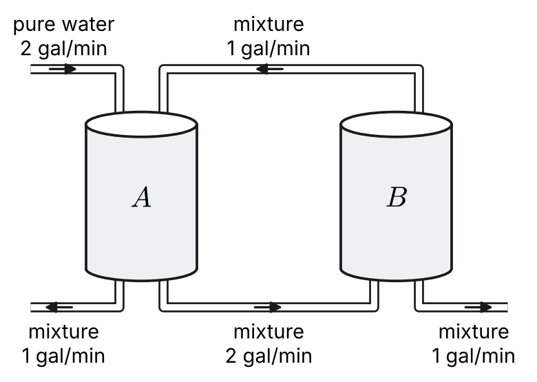
Two connected tanks, $A$ on the left and $B$ on the right. Pure water flows into tank $A$ at 2 gal/min. Mixture is pumped from tank $A$ to tank $B$ at 2 gal/min, and from tank $B$ back to tank $A$ at 1 gal/min. Mixture drains out of tank $A$ at 1 gal/min and out of tank $B$ at 1 gal/min.