← Back to Math 055

5.2 Linear Models: Boundary-Value Problems: Class Notes

5.2a

Consider $y″+3y=0,y(0)=0,y(\pi )=0$

This is a boundary-value problem (BVP) because the conditions are given at two different points, $x=0$ and $x=\pi$.

There is always the trivial solution $y=0$. We can find that

$$y=a\cos \left(\sqrt{3}x\right)+b\sin \left(\sqrt{3}x\right)$$

Since $y(0)=0$, $a=0$. Then

$$y(\pi )=0⟹b\sin \left(\sqrt{3}\pi \right)=0⟹b=0$$

($\sin \left(\sqrt{3}\pi \right)\ne 0$, because $\sqrt{3}$ is not an integer.) We only have the trivial solution.

Now consider $y″+4y=0,y(0)=0,y(\pi )=0$

$$m^2+4=0⟹m=\pm 2i⟹y=a\cos 2x+b\sin 2x$$

$$y(0)=0⟹a=0⟹y=b\sin 2x$$

$y(\pi )=0$ holds for every $b\in ℝ$, since $\sin 2\pi =0$.

$y=b\sin 2x$ is a solution to the BVP for $b\in ℝ$. The BVP has an infinite number of solutions.

Definition

A number $\lambda$ (lambda) for which there exist nontrivial solutions to $y″+P(x)y\prime +\lambda Q(x)y=0,$ $y(a)=0,y(b)=0$ is called an eigenvalue, and a solution $y=a{y}_1+b{y}_2$ that satisfies the BVP is an eigenfunction associated with the eigenvalue $\lambda$.

In the previous example, $P(x)=0$, $Q(x)=1$, $\lambda =4$ is the eigenvalue, and $y=b\sin 2x$, $b\in ℝ$, is the eigenfunction.

In the first example, $y″+3y=0$, $\lambda =3$ is not an eigenvalue: that BVP has only the trivial solution. We generalize this:

Example

Determine eigenvalues and eigenfunctions for $y″+\lambda y=0,$ $y(0)=0,y(L)=0(L>0)$.

Solution

Case I: $\lambda =0$. Then $y=ax+b$, and the boundary conditions give $a=b=0$, the trivial solution. No eigenvalues here.

Case II: $\lambda <0$. Now let $\lambda =-{\alpha }^2$, so

$$y″-{\alpha }^{2}y=0⟹m^2-{\alpha }^2=0$$

$$m=\pm \alpha ⟹y=a{e}^{\alpha x}+b{e}^{-\alpha x}$$

$y(0)=0$ gives $a=0$ (since $\cosh 0=1$). Then $y(L)=0$ gives $b\sinh \alpha L=0$, and $\sinh \alpha L\ne 0$, so $b=0$.

Again, only the trivial solution. No eigenvalue.

Case III: $\lambda >0$. Say $\lambda ={\alpha }^2$.

$$y″+{\alpha }^{2}y=0⟹m=\pm \alpha i$$

$$y=a\cos \alpha x+b\sin \alpha x$$

$y(0)=0$ gives $a=0$. Then $y(L)=0$ yields

$$b\sin \alpha L=0$$

This is true (for $b\ne 0$) whenever $\alpha L=n\pi$, $n\in {\mathbb{Z}}^{+}$. Assuming $\alpha >0$ and $L>0$,

$${\displaystyle \alpha =\frac{n\pi }{L}⟹\lambda ={\alpha }^2=\frac{n^2{\pi }^2}{L^2}}$$

This gives an infinite sequence of eigenvalues ${\displaystyle {\lambda }_n=\frac{n^2{\pi }^2}{L^2}}$, $n=1,2,3,\dots$, with eigenfunctions $y=b\sin \frac{n\pi x}{L}$ ($b\ne 0$).

5.2b

Consider a vertical beam of length $L$ with load $P$ applied to one end or a road with compressive force $P$ applied to one end. Theory of elasticity provides the differential equation ${\displaystyle EI\frac{d^{2}y}{d{x}^2}=-Py}$ or ${\displaystyle EI\frac{d^{2}y}{d{x}^2}+Py=0}$ which in standard form is

$${\displaystyle \frac{d^{2}y}{d{x}^2}+\frac{P}{EI}y=0}$$

The product $EI$ is the flexural rigidity of the beam, $E$ is Young’s modulus of elasticity, and $I$ is the moment of inertia of a cross-section of the beam (the shape’s inherent resistance to bending).

Considering $P(x)=0$, $Q(x)=1$, and letting ${\displaystyle \lambda =\frac{P}{EI}}$, this has the form

$$y″+\lambda y=0$$

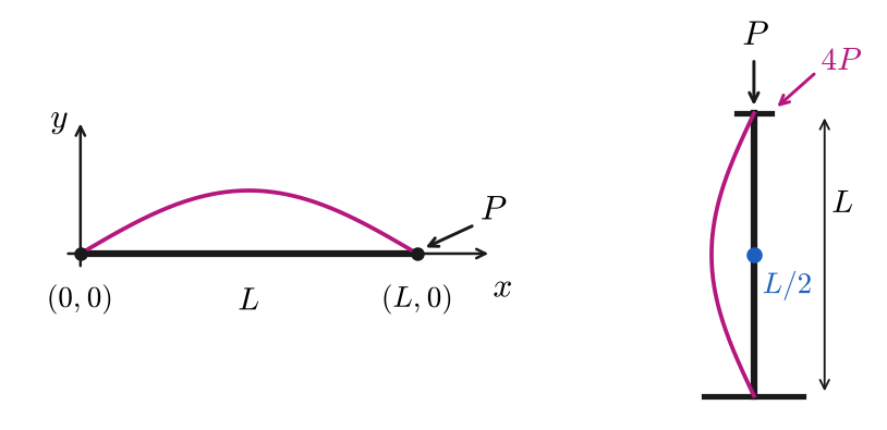
Left: a horizontal beam of length $L$ along the $x$-axis from $(0,0)$ to $(L,0)$, held at both ends, with a compressive force $P$ pushing on the end at $(L,0)$. The buckled beam (in magenta) bows into a single arch, staying at $0$ at both ends. Right: a vertical column of length $L$ with load $P$ pressing down on the top. The buckled shape (in magenta) bows out to one side, fixed at the top and bottom. A blue dot marks the midpoint $L/2$, where a support can be added; with that support, it takes a load of $4P$ to buckle the column.

With the substitution ${\displaystyle \lambda =\frac{P}{EI}}$, and considering $y(0)=0$, $y(L)=0$, we have solutions $y=b\sin \left(\frac{n\pi x}{L}\right)$ (from the eigenvalues ${\displaystyle {\lambda }_n=\frac{n^2{\pi }^2}{L^2}}$ above).

So the column/road will buckle (deflect) if

$${\displaystyle P=\frac{n^2{\pi }^{2}EI}{L^2}}$$

When $n=1$, we have the first buckling load, ${\displaystyle P=\frac{{\pi }^{2}EI}{L^2}}$.

If we restrain (support) the system at $L/2$, then the smallest critical (buckling) load will be the $n=2$ load:

$${\displaystyle P=\frac{4{\pi }^{2}EI}{L^2}}$$

That is four times the first buckling load.

Considering a beam of length $L$, the bending moment (response or resistance to load) $M(x)$ is related to the load per unit length $w(x)$ by ${\displaystyle \frac{d^{2}M}{d{x}^2}=w(x)}$ (this is from theory of elasticity). Assuming down is positive, $M(x)=EI\kappa$ is proportional to the curvature of the elastic curve. From multivariable calculus, curvature is ${\displaystyle \kappa =\frac{y″}{{[1+(y\prime {)}^2]}^{3/2}}}$. For small deflection, $y\prime \approx 0$, so $M=EIy″$. We see that $M″=w(x)$ becomes

$${\displaystyle EI\frac{d^{4}y}{d{x}^4}=w(x)}$$

Definition

The graph of the function $y(x)$ is the deflection curve of the beam.

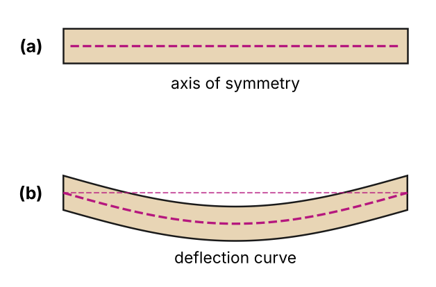
(a) A straight, unloaded beam, with its axis of symmetry drawn as a dashed line along its middle. (b) The same beam bent under a load: the dashed axis of symmetry now sags into a curve, the deflection curve. (After figures in the textbook.)

For the deflection $y(x)$, we have the following:
$y\prime$ is the slope of the curve;
a nonzero multiple of $y″$ is the bending moment ($M=EIy″$);
$\mathrm{a\; nonzero\; multiple\; of\; y}‴$ is the shear force .

The shear force is the rate of change of the bending moment:

$${\displaystyle \frac{dM}{dx}=EI\frac{d^{3}y}{d{x}^3}}$$

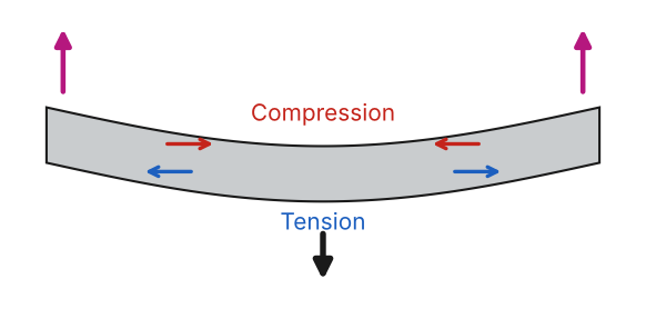
Compression and tension in a bending beam. The beam is pushed up at both ends (magenta arrows) and pulled down in the middle (black arrow), so it bends. Along the top of the beam the material is squeezed together (compression, arrows pointing toward the middle); along the bottom it is stretched apart (tension, arrows pointing toward the ends).

If the end of the beam is

• embedded, $y=0,y\prime =0$;
• free, $y″=0,y‴=0$;
• simply supported/hinged, $y=0,y″=0$.

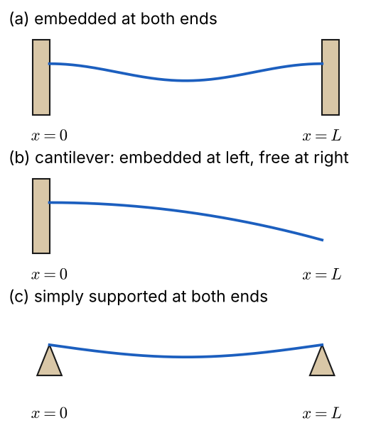
Three beams from $x=0$ to $x=L$, each with its deflection curve. (a) Embedded at both ends: both ends are built into walls, so the curve is level where it leaves each wall. (b) Cantilever: the left end is built into a wall and the right end hangs free, drooping down. (c) Simply supported: each end rests on a support point, and the beam sags between them. (After a figure in the textbook.)

5.2c

Example

Solve the differential equation ${\displaystyle EI\frac{d^{4}y}{d{x}^4}=w(x)}$ subject to the appropriate boundary conditions. The beam is of length $L$, and $w_0$ is a constant.

(a) The beam is simply supported at both ends, and $w(x)=w_0,0<x<L$.

Solution

Simply supported at both ends means $y=0$ and $y″=0$ at each end:

$$y(0)=0,y(L)=0,y″(0)=0,y″(L)=0$$

Divide by $EI$ and integrate four times:

$${\displaystyle \begin{array}{cc}\hfill {\displaystyle \frac{d^{4}y}{d{x}^4}}& {\displaystyle =\frac{w_0}{EI}}\hfill \\ \hfill {\displaystyle y‴}& {\displaystyle =\frac{w_0}{EI}x+c_1}\hfill \\ \hfill {\displaystyle y″}& {\displaystyle =\frac{w_0}{2EI}{x}^2+c_{1}x+c_2}\hfill \\ \hfill {\displaystyle y\prime }& {\displaystyle =\frac{w_0}{6EI}{x}^3+\frac{c_1}{2}{x}^2+c_{2}x+c_3}\hfill \\ \hfill {\displaystyle y}& {\displaystyle =\frac{w_0}{24EI}{x}^4+\frac{c_1}{6}{x}^3+\frac{c_2}{2}{x}^2+c_{3}x+c_4}\hfill \end{array}}$$

$y(0)=0⟹c_4=0$ and $y″(0)=0⟹c_2=0$, so

$${\displaystyle y=\frac{w_0}{24EI}{x}^4+\frac{c_1}{6}{x}^3+c_{3}x}$$

$${\displaystyle \begin{array}{cc}\hfill {\displaystyle y(L)=0}& {\displaystyle ⟹0=\frac{w_0}{24EI}{L}^4+\frac{c_1}{6}{L}^3+c_{3}L}\hfill \\ \hfill {\displaystyle y″(L)=0}& {\displaystyle ⟹0=\frac{w_0}{2EI}{L}^2+c_{1}L}\hfill \end{array}}$$

The second equation gives ${\displaystyle c_1=-\frac{w_{0}L}{2EI}}$. Substituting into the first, ${\displaystyle 0=\frac{w_0{L}^4}{24EI}-\frac{w_0{L}^4}{12EI}+c_{3}L}$, so ${\displaystyle c_3=\frac{w_0{L}^3}{24EI}}$. We find that

(b) Use a graphing utility to graph the deflection curve when $w_0=24EI$ and $L=1$.

Solution

Then ${\displaystyle \frac{w_0}{24EI}=1}$, so

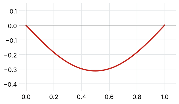
Graph of $-y=-(x^4-2x^3+x)$ for $0\le x\le 1$ (in red). Since down is positive, the deflection is plotted as $-y$ so that the beam sags below the axis. The curve starts at $(0,0)$, dips to its lowest point $(0.5,-0.3125)$ at the middle of the beam, and comes back to $(1,0)$; it is symmetric about $x=0.5$.