2.1 Solution Curves Without a Solution: Class Notes

2.1a

Definition

If $y = y (x)$ is a differentiable function, then $\frac{d y}{d x}$ gives the slope of a tangent line at a point. We can learn about a DE $\frac{d y}{d x} = f (x, y)$ using segments of tangent lines, called lineal elements. The collection of these lineal elements is a direction field or slope field.

Example

Sketch an approximate solution curve that passes through each of the indicated points

$\frac{d y}{d x} = x^{2} - y^{2}$

a) $y (- 2) = 1$ b) $y (3) = 0$ c) $y (0) = 2$ d) $y (0) = 0$

Start at each given point and follow the lineal elements in both directions: the curve runs parallel to the nearby segments everywhere. Each curve below is drawn in the same color as its initial condition.

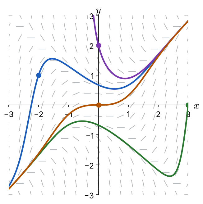
Direction field for dy/dx = x squared minus y squared with four solution curves

Direction field on $- 3 \leq x \leq 3$ , $- 3 \leq y \leq 3$ with four solution curves. a) Through $(- 2, 1)$ : rises steeply from the lower left, peaks near $(- 1.6, 1.6)$ , dips to a low point near $(0.5, 0.5)$ , then climbs along the line $y = x$ to the upper right. b) Through $(3, 0)$ : comes up from the lower left to a high point near $(- 0.5, - 0.5)$ , falls to a low point near $(2.4, - 2.4)$ , then shoots up steeply to $(3, 0)$ . c) Through $(0, 2)$ : comes down steeply from the top just left of the $y$ -axis, reaches a low point near $(0.9, 0.9)$ , then climbs along $y = x$ . d) Through $(0, 0)$ : rises from the lower left along $y = x$ , levels off with a horizontal tangent at the origin, then climbs along $y = x$ to the upper right.

Example

Use computer software to obtain a direction field for the differential equation. Sketch an approximate solution curve passing through each of the given points.

$y' = x + y$

a) $y (- 2) = 2$ b) $y (1) = - 3$

Direction field for y prime = x + y with two solution curves

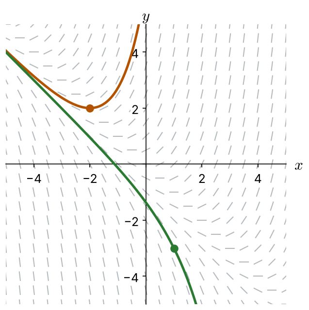
Direction field on $- 5 \leq x \leq 5$ , $- 5 \leq y \leq 5$ with two solution curves. a) Through $(- 2, 2)$ : a U-shaped curve whose lowest point is $(- 2, 2)$ itself; it rises to the left along the line $y = - x - 1$ and rises steeply to the right. b) Through $(1, - 3)$ : decreases everywhere, following the line $y = - x - 1$ on the left and dropping steeply to the right.

2.1b

Definition

A DE in which the independent variable does not appear explicitly is an autonomous differential equation. A first-order autonomous DE has the form $\frac{d y}{d x} = f (y)$ .

For example, $\frac{d P}{d t} = k (P - 5)$ is autonomous: the independent variable $t$ does not appear on the right side.

Definition

A number $c$ is a critical point of an autonomous DE if $f (c) = 0$ . A critical point is also known as an equilibrium point or stationary point. A constant solution $y (x) = c$ of an autonomous DE is an equilibrium solution.

In the example above, $k (P - 5) = 0$ when $P = 5$ , so $P = 5$ is a critical point and $P (t) = 5$ is an equilibrium solution.

Example

Consider the autonomous first-order differential equation $\frac{d y}{d x} = y^{2} - y^{4}$ and the initial condition $y (0) = y_{0}$ . Sketch the graph of a typical solution $y (x)$ when $y_{0}$ has the given values.

a) $y_{0} > 1$ b) $0 < y_{0} < 1$ c) $- 1 < y_{0} < 0$ d) $y_{0} < - 1$

Solution

Find the critical points by setting $\frac{d y}{d x} = 0$ :

$\begin{matrix} y^{2} - y^{4} & = 0 \\ y^{2} (1 - y^{2}) & = 0 \\ y^{2} (1 + y) (1 - y) & = 0 \end{matrix}$

The critical points are $y = - 1$ , $y = 0$ , and $y = 1$ . They give the equilibrium solutions $y = - 1$ , $y = 0$ , and $y = 1$ (horizontal lines). Next, find the sign of $y' = y^{2} (1 + y) (1 - y)$ between and beyond the critical points. The factor $y^{2}$ is never negative, so the sign comes from $(1 + y) (1 - y)$ :

Sign of the derivative in each region
$y_{0}$	$sign of y'$	$solution$
$y_{0} > 1$	$y' < 0$	$decreasing$
$0 < y_{0} < 1$	$y' > 0$	$increasing$
$- 1 < y_{0} < 0$	$y' > 0$	$increasing$
$y_{0} < - 1$	$y' < 0$	$decreasing$

A solution can never cross an equilibrium solution, so each typical solution stays between the same pair of horizontal lines (or beyond the outer one) and levels off toward them:

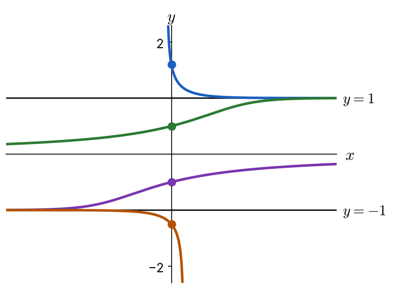
Typical solution curves of dy/dx = y squared minus y to the fourth, for four ranges of y sub 0

Equilibrium solutions $y = 1$ , $y = 0$ (the $x$ -axis), and $y = - 1$ . a) For $y_{0} > 1$ , the curve decreases toward $y = 1$ as $x \to \infty$ and rises steeply to the left. b) For $0 < y_{0} < 1$ , the curve increases from near $y = 0$ on the left toward $y = 1$ on the right. c) For $- 1 < y_{0} < 0$ , the curve increases from near $y = - 1$ on the left toward $y = 0$ on the right. d) For $y_{0} < - 1$ , the curve decreases from near $y = - 1$ on the left and drops steeply downward to the right.

This information can be collapsed into a one-dimensional graph, called a phase portrait: a vertical $y$ -axis with the critical points marked and arrows showing whether solutions increase (up) or decrease (down) in each region.

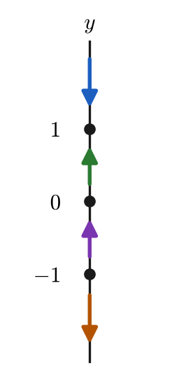
Phase portrait for dy/dx = y squared minus y to the fourth with critical points minus 1, 0, and 1

Vertical $y$ -axis with dots at $y = - 1$ , $0$ , and $1$ . Arrows: pointing down above $1$ ; pointing up between $0$ and $1$ ; pointing up between $- 1$ and $0$ ; pointing down below $- 1$ .

Reading the arrows near each critical point:

• $1$ is an attractor (asymptotically stable): the arrows on both sides point toward it.

• $0$ is semi-stable: the arrows on both sides point up, toward it from below and away from it above.

• $- 1$ is a repeller (unstable): the arrows on both sides point away from it.